This nimib example document shows how to insert images in nimib documents.
🐧 Exploring penguins with ggplotnim
We will explore the palmer penguins dataset with ggplotnim and datamancer.
import datamancerwe read the penguins csv into a Datamancer DataFrame
let df = readCsv("data/penguins.csv")let us see how it looks
echo dfDataFrame with 7 columns and 344 rows:
Idx species island culmen_length_mm culmen_depth_mm flipper_length_mm body_mass_g sex
dtype: string string object object object object string
0 Adelie Torgersen 39.1 18.7 181 3750 MALE
1 Adelie Torgersen 39.5 17.4 186 3800 FEMALE
2 Adelie Torgersen 40.3 18 195 3250 FEMALE
3 Adelie Torgersen NA NA NA NA NA
4 Adelie Torgersen 36.7 19.3 193 3450 FEMALE
5 Adelie Torgersen 39.3 20.6 190 3650 MALE
6 Adelie Torgersen 38.9 17.8 181 3625 FEMALE
7 Adelie Torgersen 39.2 19.6 195 4675 MALE
8 Adelie Torgersen 34.1 18.1 193 3475 NA
9 Adelie Torgersen 42 20.2 190 4250 NA
10 Adelie Torgersen 37.8 17.1 186 3300 NA
11 Adelie Torgersen 37.8 17.3 180 3700 NA
12 Adelie Torgersen 41.1 17.6 182 3200 FEMALE
13 Adelie Torgersen 38.6 21.2 191 3800 MALE
14 Adelie Torgersen 34.6 21.1 198 4400 MALE
15 Adelie Torgersen 36.6 17.8 185 3700 FEMALE
16 Adelie Torgersen 38.7 19 195 3450 FEMALE
17 Adelie Torgersen 42.5 20.7 197 4500 MALE
18 Adelie Torgersen 34.4 18.4 184 3325 FEMALE
19 Adelie Torgersen 46 21.5 194 4200 MALE
or even nicer using nbShow(df.head(10)):
| Index | species string | island string | culmen_length_mm object | culmen_depth_mm object | flipper_length_mm object | body_mass_g object | sex string |
|---|---|---|---|---|---|---|---|
| 0 | Adelie | Torgersen | 39.1 | 18.7 | 181 | 3750 | MALE |
| 1 | Adelie | Torgersen | 39.5 | 17.4 | 186 | 3800 | FEMALE |
| 2 | Adelie | Torgersen | 40.3 | 18 | 195 | 3250 | FEMALE |
| 3 | Adelie | Torgersen | NA | NA | NA | NA | NA |
| 4 | Adelie | Torgersen | 36.7 | 19.3 | 193 | 3450 | FEMALE |
| 5 | Adelie | Torgersen | 39.3 | 20.6 | 190 | 3650 | MALE |
| 6 | Adelie | Torgersen | 38.9 | 17.8 | 181 | 3625 | FEMALE |
| 7 | Adelie | Torgersen | 39.2 | 19.6 | 195 | 4675 | MALE |
| 8 | Adelie | Torgersen | 34.1 | 18.1 | 193 | 3475 | NA |
| 9 | Adelie | Torgersen | 42 | 20.2 | 190 | 4250 | NA |
Note that among the 7 columns of the dataframe, the first 2 and the last one have datatype string. The remaining 4 are numeric but they have datatype object. Why?
Because that there are null values in those columns (interpreted as strings):
echo df["culmen_depth_mm", 1].kind
echo df["culmen_depth_mm", 2].kind
echo df["culmen_depth_mm", 3].kind
echo df["flipper_length_mm", 2].kind
echo df["flipper_length_mm", 3].kind
VFloat VFloat VString VInt VString
Let's see how many penguins by species we have (and how do they relate to islands) by plotting the species count per island using ggplotnim:
import ggplotnim
ggplot(df, aes("species", fill = "island")) + geom_bar() + ggsave("images/penguins_count_species.png")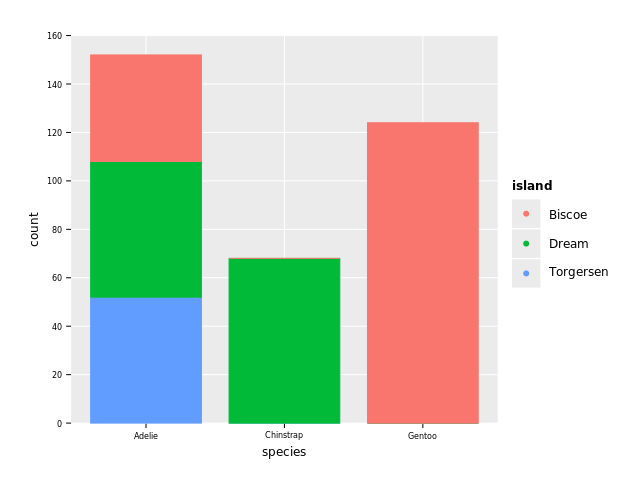
We see that 3 species of penguins (Adelie, Chinstrap, Gentoo) are reported living on 3 islands (Biscoe, Dream, Torgersen). The majority of penguins are Adelie and they are distributed over the 3 islands. Gentoo penguins (second most common) almost all live on Biscoe, and Chinstrap penguins almost all live on Dream.
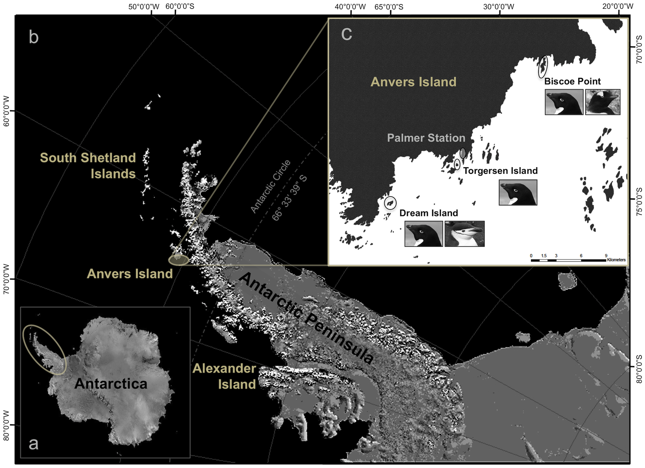
We can confirm this with the following image taken from the article from where this dataset comes from:
We do expect weight being correlated to some of the length measures (e.g. flipper length) with males being bigger than females.
To plot this we need to remove all NA and then classify the points both by the penguins sex as
well as their species:
let df1 = df.filter(f{`body_mass_g` != "NA"}) # c"foo" == `foo` == idx("foo") (backtick quotes not usable for columns with spaces)
ggplot(df1, aes(x="body_mass_g", y="flipper_length_mm", color = "sex", shape="species")) + geom_point() + ggsave("images/penguins_mass_vs_length_with_sex.png")
INFO: The object column `body_mass_g` has been automatically determined to be continuous. To overwrite this behavior use `scale_x/y_discrete` or apply `factor` to the column name in the `aes` call. INFO: The object column `flipper_length_mm` has been automatically determined to be continuous. To overwrite this behavior use `scale_x/y_discrete` or apply `factor` to the column name in the `aes` call.
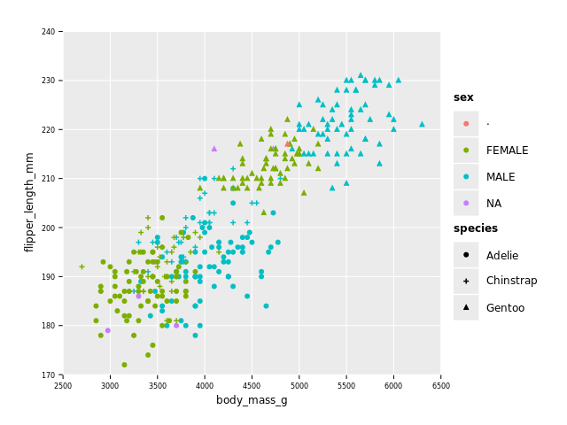
A few things to remark:
- as expected body mass and flipper length are linearly correlated
- males are in general bigger than females but there appear 2 groups, possibly related to species
- we have some more NAs (and one '.') in sex column (even after filtering for NAs in numeric columns)
- we can see that sizes of Adelie and Chinstrap overlap, while Gentoo penguins are in general bigger
As a final plot, I would like to (partly, confidence bands are missing) reproduce a plot that "shows" the presence of Simpson's paradox in this dataset, as reported by this tweet:
ggplot(df1, aes(x="culmen_depth_mm", y="body_mass_g")) +
  geom_point(aes = aes(color = "species")) +      # point...
  geom_smooth(aes = aes(color = "species"),       # and smooth classified by species
              smoother = "poly", polyOrder = 1) + # polynomial order 1 == line
  geom_smooth(smoother = "poly", polyOrder = 1) + # and smooth without classification by species
  ggsave("images/penguins_simpson.png")
INFO: The object column `culmen_depth_mm` has been automatically determined to be continuous. To overwrite this behavior use `scale_x/y_discrete` or apply `factor` to the column name in the `aes` call. INFO: The object column `body_mass_g` has been automatically determined to be continuous. To overwrite this behavior use `scale_x/y_discrete` or apply `factor` to the column name in the `aes` call.
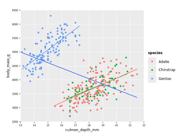
We can see that Gentoo penguins, although in general bigger, have a "thinner" bill (see image below for meaning of bill and culmen)!
